
There are two main types of Data Warehouses: OLAP (Online Analytical Processing) and OLTP (Online Transactional Processing).
The first one is designed to be used by data analysts, business managers, where data is constantly updated in batch, to allow decision making. The latter is designed to control and run essential business operations in real time and the updates are fast, but in smaller amount.
In terms of historical information, OLAP provides multi-dimensional view of the whole data available in a company where as OLTP concatenates daily transactions, for example.
It is a OLAP solution and and it works as follows:
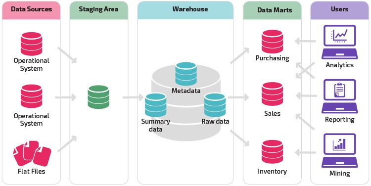
Extracted from: https://datawarehouseinfo.com/wp-content/uploads/2018/09/DW-architecture.jpg
Generally speaking, a DW stores 3 types of data (summary data, raw data and metadata), which are derived from many sources and these data can be split into different data marts depending on the goal, in order to support decision making and help solve business problems. In Staging, it is where we create the ETL layer, responsible for transforming data the way we need
It is a serverless data warehouse, that can scale and has high-availability depending on our needs! It is a DW solution provided by Google and it is charged based on demand.
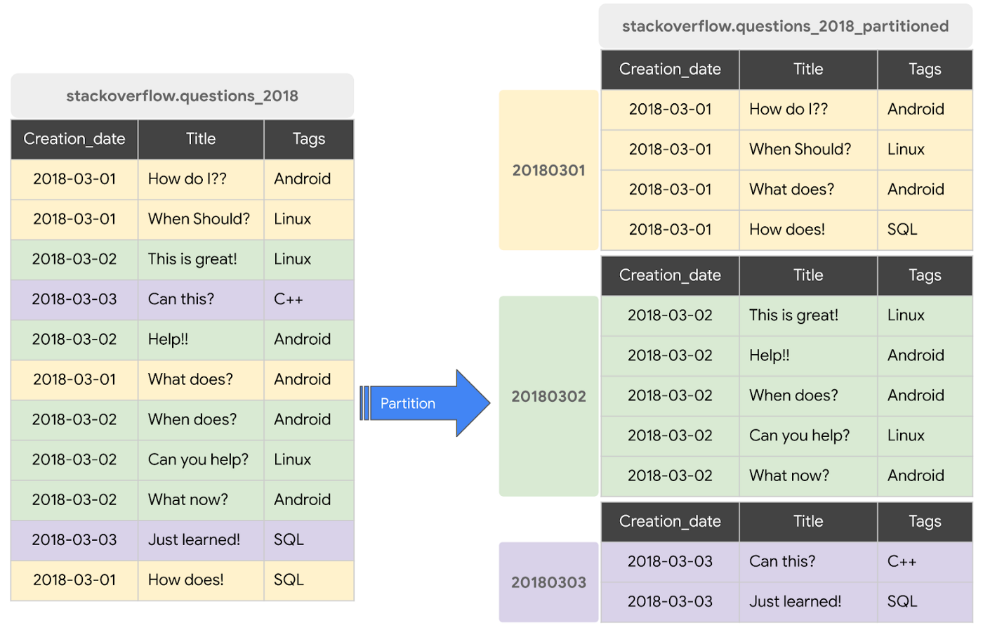
Imagine we have raw data , based on questions posted on StackOverflow and these question are marked with their creation date, title and tags. If we only want to query questions made on March 2nd 2018, BigQuery will have to look for every row and filter out only those from March 2nd 2018, which is an expensive task, depending on how much data we have. However, here comes partitioning: we can create the same table partitioned by the creation data, so that BQ will find our desired data much faster and cost us less, like below:

Extracted from: https://storage.googleapis.com/gweb-cloudblog-publish/images/BigQuery_Explained_Storage_5.max-1400x1400.png
From our previous section, we saw that we are able to partition our data in such a way that our queries becomes faster and light-weighted, reducing our costs! Additionally, we can create one more level of compactness, by clustering the data inside the partitions. So, in our previous image, we can see that on March 2nd 2018, we have questions for Android and Linux and this way, we can cluster these 5 rows by Tags, that would make our first 3 rows as being Android and the last 2 rows as being Linux, optimizing our further queries.
NOTE: tables sizes less than 1GB, partitioning and clustering don’t show significant improvement